Siddharth Saha | Paper Review: MILP Models for Multi-Robot Non-Adversarial Search

My implementation is available on this GitHub repo

In One Line

This paper¹ attempts to solve the Multi-robot Efficient Search Path Planning problem using Mixed Integer Linear Programming

Contrasting with Previous Work

The original paper by Hollinger² used sequential allocation and receding-horizon planning. In this paper, the proposed MILP models for the MESPP problem allow path enumeration to be performed in a much more efficient way by leveraging the sophisticated branching and pruning techniques of modern MILP solvers.

Pre-requisite Terminology

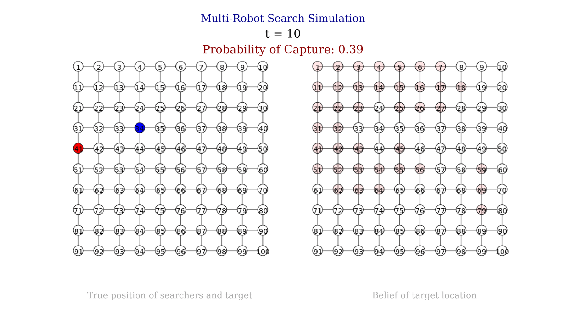
MESPP

In Multi-robot Efficient Search Path Planning (MESPP), a team of robots is tasked with capturing a moving target within a given deadline.

Non-adversarial

In this paper, we assume that the target is non-adversarial. This simply means that the target doesn’t try to foil the capture team’s plans and sticks to its pre-defined course of actions.

NP-Hard

NP-Hard problems are a class of problems, for which no polynomial-time algorithms are known to exist as yet. An NP-Hard problem can be reduced to any other problem in the NP-Hard class of problems in polynomial time. Once the given problem is proven to be NP-Hard, we can convert it to more familiar versions of NP-Hard problems for which (non-polynomial time) algorithms are known.

MILP

Mixed Integer Linear Programming (MILP) is an optimization problem where only some variables are constrained to be integers, while other variables can be non-integers. It deals with linear objective function subjected to linear constraints.

Explicit Coordination

All robots participate in the path-planning for all robots (thus, planning in the joint path space).

Implicit Coordination

Multiple robots share information and plan for themselves rather than planning in the joint path space.

False Negatives

Target was present within sensing range but the capture robot missed it.

Arbitrary Capture Ranges vs Same Vertex Capture

How far the capture robot’s sensing range can reach. Analogously, how close the capture team robots need to be to the moving target to declare the target as captured.
Single vertex capture means that the searcher and object must be on the same vertex to declare that target has been captured.

Environment Representation

We use $G = (V, E)$, as an undirected, connected, and simple graph representing a known environment with $V = {1, 2, . . ., n}$
There are $n$ vertices; Discrete time intervals; There are $m$ searchers

Optimization Problem: Objective

\[\mathbf{\pi^*} = argmax_{\pi \in P} \sum_{t=0}^{\tau} \gamma^t b_c(t)\]

$\mathbf{\pi^*}$: We’re trying to optimize the path taken by ALL searchers to maximize our probability of capturing the target at the earliest time.
Let’s say we capture the target much before the deadline $\tau$, $b_c(t)$ will become 1 for the remaining time duration, automatically becoming the optimal solution
$P$: set of all possible joint paths across all searchers
$\gamma^t$: $\gamma$ is discount factor (Discounting is done by raising to time t)
$\gamma$ is a number less than 1, the purpose is to give greater weight to finding the object sooner.

Optimization Problem: Constraints

Legal Path for Searchers

\[x_v^{s,t} \in \{0,1\}, \forall s \in S, (v,t) \in V^{s,t}\] \[y_{uv}^{s,t} \in \{0,1\}, \forall s \in S, (u,t < \tau) \in V^{s,t}, v \in \delta'(u)\] \[y_{uv_g}^{s,\tau} \in \{0,1\}, \forall s \in S, u \in V^{s,t}(\tau)\]

$x_v^{s,t}$ and $y_{uv}^{s,t}$ are binary variables
$x_v^{s,t} = 1$ denotes presence of searcher $\textbf{s}$ in vertex $\textbf{v}$ at time t
$y_{uv}^{s,t} = 1$ denotes the searcher $\textbf{s}$ will move from $\textbf{u}$ to $\textbf{v}$ in [t,t+1]
$\delta(v)$ denotes the neighbors of $v \in V$ and $\delta’(v)$ denotes $\delta(v) \cup {v}$
$v_g$ is explained below

\[x_{v_o^s}^{s,0} = 1 = \sum_{ j \in \delta'(v_o^s)} y_{v_o^s j}^{s,0} = \sum_{ j \in V^{s,t}(\tau)} y_{j v_g}^{s,\tau}, \forall s \in S\] \[x_v^{s,t} = \sum_{ j \in \delta'(v) \,\cap\, V^{s,t}(t-1) } y_{j v}^{s,t-1} = \sum_{ i \in \delta'(v)} y_{v i}^{s,t}, \forall (v,t < \tau) \in V^{s,t}\] \[x_v^{s,\tau} = \sum_{ j \in \delta'(v) \,\cap\, V^{s,t}(\tau-1) } y_{j v}^{s,\tau-1} = y_{v v_g}^{s,\tau}, \forall (v,t < \tau) \in V^{s,t}(\tau)\]

The first constraint:
- Presence of searcher s at its start location is 1 (by definition)
- The second equality forces the searcher s to take some action, whether stay in the same vertex $v_o^s$ or move to any of its neighbors
- The last equality refers to a fictitious vertex $v_g$ that we introduce to ensure that all searchers leave the world at the deadline $\tau$. We assume $v_g$ is connected to all vertices at the deadline.
The second constraint:
- If a searcher s is present in vertex v at time t, the presence variable will become 1
- Simultaneously, we ensure that it had entered vertex v from legitimate edge-sharing vertices in the previous time step
- Also ensures that the searcher exits the vertex v legally and if presence variable is 1, the searcher picks exactly 1 destination
The third constraint:
- Rules at the deadline or time horizon
- The exit rule is special, it is forced to enter the fictitious goal vertex (thus exiting the world)

Target’s Motion

\[\beta_i^t \in [0,1], \forall i \in V \cup \{c\}, t \in \{0\} \cup T\] \[\alpha_v^t \in [0,1], \forall v \in V, t \in T\]

$\beta_i^t$ - entry of the belief vectors at time t
$\alpha_v^t$ - result of the application of the motion model

\[\beta_i^0 = b_i(0), \forall i \in V \cup \{c\}\] \[\alpha_v^t = \sum_{u \in V} \mathbf{M}_{uv} \beta_u^{t-1}, \forall v\in V, t\in T\]

Here we talk about the belief propagation at any time instant t using a motion model. We can see from the second equation that $\alpha$ is being evolved from the previous belief $\beta$
$\mathbf{M}$ represents a known motion model of the object. It is an $n\times n$ matrix, where $\mathbf{M}_{uv}$ denotes the probability that the object will move from u to v in time interval $[t,t+1]$. This has been referred to as the dispersion model $\mathbf{D}$ in the original paper by Hollinger²

Capture Events in Same Vertex, Binary Detection

We introduce another binary variable, $\psi_v^t = 1 \iff \exists$ atleast one searcher is located in v at t

\[\beta_v^t = \alpha_v^t (1-\psi_v^t), \forall t \in T, v \in V\]

If at least one searcher is present in vertex v, we assume the worst (no target present) and update the belief as 0
Note that we’re planning for the future, so we have not actually moved t steps into the future and done a real observation
If no searcher is present in vertex v, the best that we can predict is from the belief propagation using the motion model

The model is non linear so we linearize it as follows

\[\beta_v^t \leq 1-\psi_v^t\] \[\beta_v^t \leq \alpha_v^t\] \[\beta_v^t \geq \alpha_v^T - \psi_v^t\] \[\psi_v^t \in \{0,1\}\]

The beauty in the above linearization is if you substitute $\psi_v^t$ as 0 or 1, the result is same from the non-linear equation and the linear formulation. (If you’re working this out, keep in mind that $\beta_v^t$ is lower bounded at 0)

If all searchers are in vertex v at time t, $\psi_v^t$ = 1 then equality holds

\[\sum_{s \in S\, s.t.\, v\in V^{s,t}(t)} x_v^{s,t} \leq m\psi_v^t, \forall v\in V, t\in T\]

If however no searcher is in v equality holds

\[\psi_v^t \leq \sum_{s \in S \, s.t.\, v\in V^{s,t}(t)} x_v^{s,t}, \forall v\in V, t\in T\]

Probability of object getting caught of

\[\beta_c^t = 1 - \sum_{v\in V}\beta_v^{t}, \forall t \in T\]

If we have sufficiently explored all vertices where we suspect the target to be the most, the capture probability goes closer and closer to 1

Capture Events Within Given Range, Binary Detection

Just 2 equations change (related to capture). The searcher s is located at u, to detect the object within the sensing range of vertex v

\[\sum_{s \in S} \sum_{u \in V^{s,t}(t)\, s.t.\, \mathbf{C}_{v,0}^{s,u}=1} x_v^{s,t} \leq m\psi_v^t, \forall v\in V, t\in T\] \[\psi_v^t \leq \sum_{s \in S} \sum_{u \in V^{s,t}(t)\, s.t.\, \mathbf{C}_{v,0}^{s,u}=1} x_u^{s,t}, \forall v\in V, t\in T\]

$\mathbf{C}^{s,u}$ is the (n+1)✕(n+1) capture matrix. It represents which vertices of the graph fall within the sensing range of searcher s, when s is located in vertex u. The subscript refers to the location in the capture matrix

Transcription

Conversion of a complex mathematical problem into constrained parameter optimization problem.

Presolve level

Presolve is a preprocess of the Linear Programming model. It looks for ways to simplify it. For example it can delete unused variables and restrictions. Substitute fixed variable values by a constant and so on. The result is a new model that is less complex than the original model and likely solves faster.
Usually, there are less variables and/or constraints in the presolved model.